Modeling Active COVID-19 Cases with Advanced DAX in Power BI

This is the fourth post in a series on building a Power BI report on the COVID-19 data. The source of the data is the COVID-19 Data Repository by the Center for Systems Science and Engineering (CSSE) at Johns Hopkins University. This post builds on the foundation from the previous steps.

Part 1: Import COVID-19 Data with Power BI
Part 2: Create a Star Schema with COVID-19 Data in Power BI
Part 3: Create Simple Reports on COVID-19 Cases with Power BI]
Part 4: Modeling Active COVID-19 Cases with Advanced DAX in Power BI (This Post)

In the previous post we created a simple report on the COVID-19 time series data. We extended the initial count measures by adding Previous Day counts and Daily Change counts. We also added an # Active measure, which lead us to suspect some problems with the data.

Problem

Because the # Active measure we created is derived by taking the number of # Confirmed cases and subtracting # Deaths and # Recovered it, can only be as accurate as the inputs. To illustrate the problem see the following two graphs.

Slice By Germany

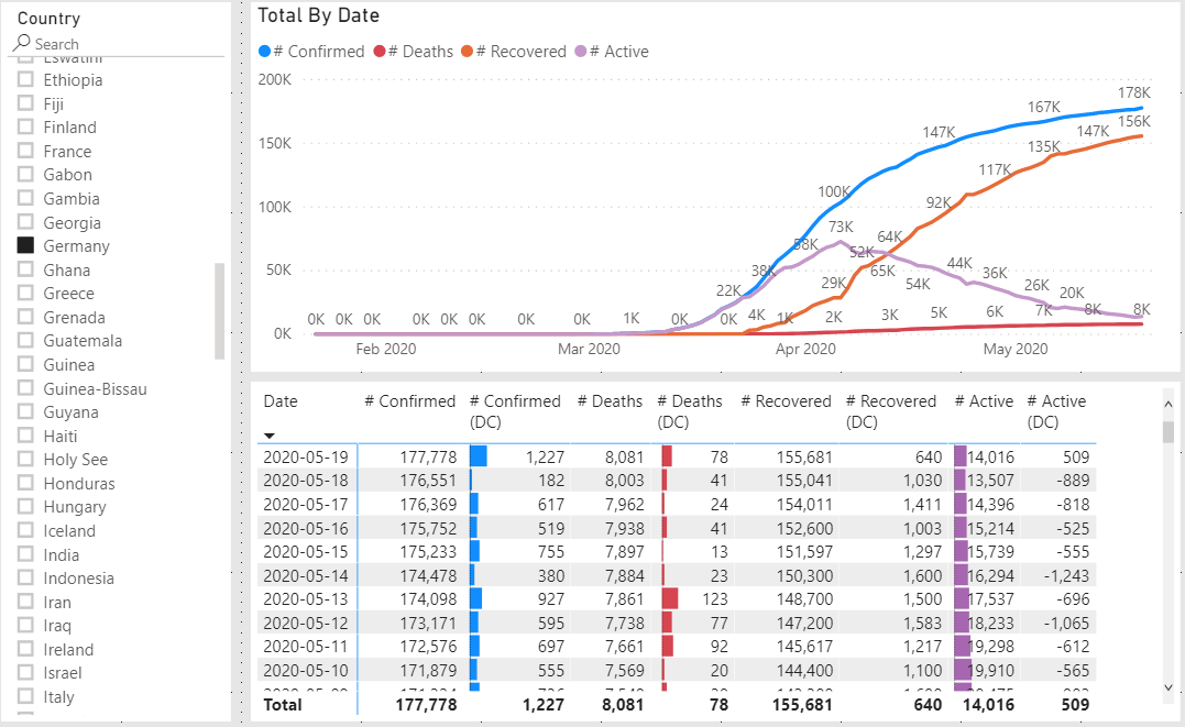
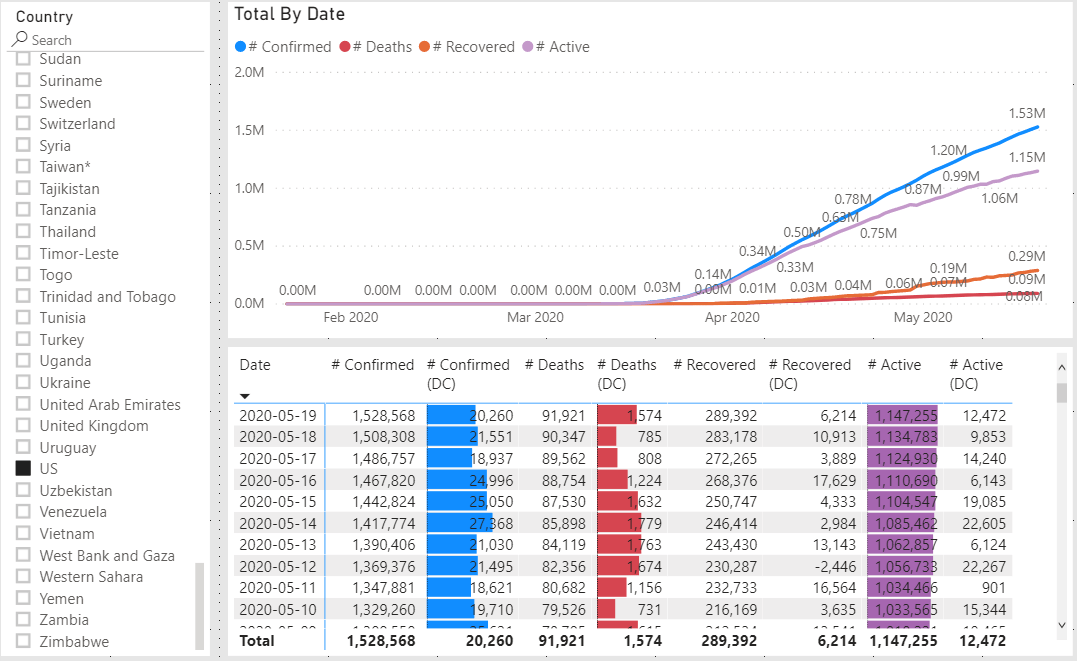Slice by United States The percent of recovered cases vs total cases in Germany is a much larger than in the United States while the number of deaths is relatively small (compared to total cases) for both. We do not need to know why it is different, only that it is different. Anything else is speculation from a data science point of view.

How long is a person able to spread the virus?

Let’s think about what happens when an individual contracts this virus. There are two possible outcomes, it may be fatal or they will recover at some point. This is not a chronic condition where the person remains sick for years. The important thing that we want to estimate is how many people are currently actively sick and able to infect others.

Discamer: I am not a medical doctor and I do not give medical advice. I am only demonstrating a relatively simple model which may help to provide insight, or at least, an interesting way to pass the time.

Doing a bit of research on COVID-19, I found these bits of information.

Of those that get symptoms, they usually show up between 2-14 days after infection.
The average recovery time for mild cases is around 14 days.

According to the CDC it is safe for a person who has been sick with COVID-19 to leave isolation after all of these conditions are met.

No fever for at least 72 hours without medication.
Other symptoms have improved.
At least 10 days since symptoms appeared.

By combining these points we derive a range of 12-24 days that a person that has symptoms and tested positive needs to isolate because they may infect others.

Unfortunately, that only covers the case where the person recovers. The fatal outcome will likely happen sometime within a smaller window. This is due to a number of factors. If a person has a bad case they could pass quickly or a mild case may not be detected as fast, but may be detected late in the cycle.

In all cases, detection happens some number of days after infection. For example, there could be a +1 to confirmed count on the patient’s day 3 of being infected. There is no way to know this information, so we will guess and subtract 3 from the 12-24 day range which gives 9-21 day range. We should also assume that the distribution over this range is going to be biased towards the latter part of the range.

Putting all of these assumptions together I came up with a distribution that looks like this.

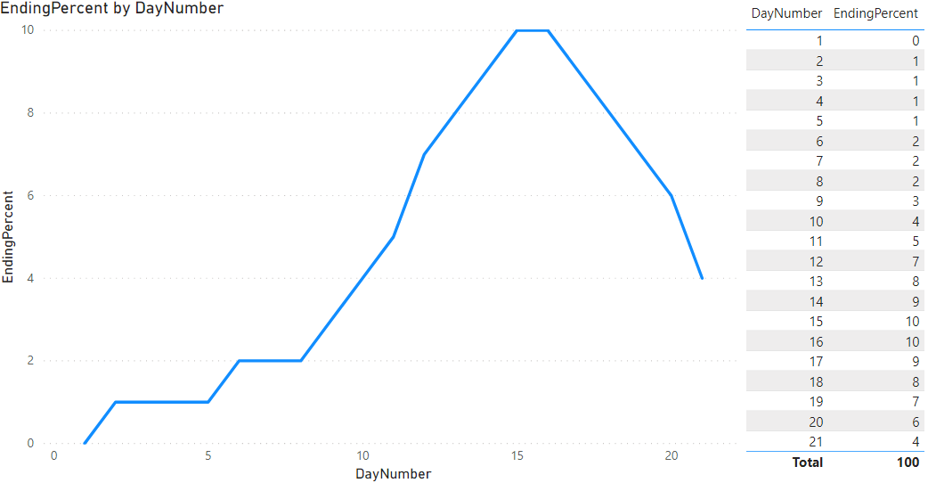Ending Percent Note, some small number of cases are early in the curve while most are after day 11. This is a starting point that can be modified later once we see how well it performs.

That’s great, but how do I use this model?

Solution

This is the fun part. Keep in mind this distribution represents cases that are finished and no longer active.

To solve complex problems like this, I like to write it out in pseudo-code.

For each day, get the number of new cases
Multiply that day by the 21 day distribution to get 21 days into the future (FinishDate)
On each of these 21 days, multiply the original number of new cases by the EndingPercent to get NumberFinished
Aggregate the NumberFinished by FinishDate

How to implement this in Power BI

We already wrote a measure to get the number of new cases, but that is at an aggregate level. We need to do the same thing again, but at a lower level within the Daily Total table.

On the Data tab, add a new calculated column to the Daily Total table.

 1
 2
 3
 4
 5
 6
 7
 8
 9
10
11
12
13
14
15


NewCases = 
VAR ThisGeographyId = 'Daily Total'[GeographyID]
VAR PreviousReportDate = PREVIOUSDAY('Daily Total'[ReportDate]) 
VAR PreviousConfirmed = 
    CALCULATE
        (
        MAX('Daily Total'[Confirmed])
        , FILTER
            (
            'Daily Total'
            , 'Daily Total'[GeographyID] = ThisGeographyId && 'Daily Total'[ReportDate] = PreviousReportDate
            )
        )
RETURN
'Daily Total'[Confirmed] - PreviousConfirmed

This new column gets the Confirmed value for the previous day (line 3) for the same geography (line 2). We change the evaluation context of the MAX(Confirmed) by using the calculate function to filter the Daily Total table to get the correct record. Line 15 does the subtraction to get the number of new cases on that date. Hide this column because we do not want report users to use it out of context.

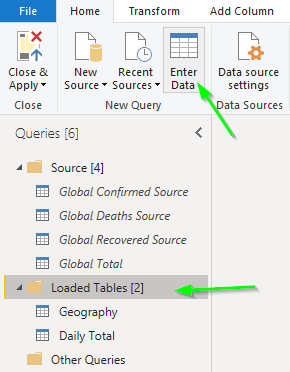
Next, we need to add the values for our model. Open Power Query by clicking on the Transform Data button. Click on the Loaded Tables group and then click the Enter Data button. Name the table End Distribution and then type these values into each column. 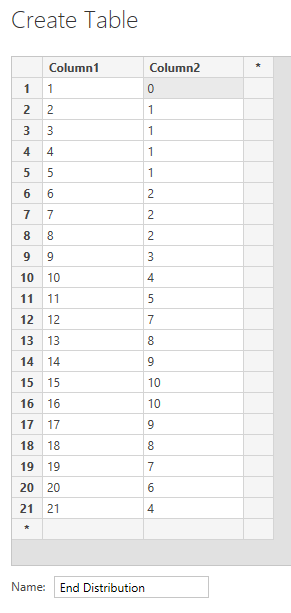Rename Column1 to DayNumber and Column2 to EndingPercent. Then click Close & Apply.

Now things get complicated. We need to multiply every row from the Daily Total table by every row on the End Distribution table. We will build this up through a series of steps.

FirstCreate a new table named ‘Finished’ by clicking New Table button while on the Data tab. Enter this code into the formula bar.

 1
 2
 3
 4
 5
 6
 7
 8
 9
10
11
12
13


Finished = 
VAR FinishedTableBase = 
        CROSSJOIN(
            SELECTCOLUMNS(
                  'Daily Total'
                , "ReportDate", 'Daily Total'[ReportDate]
                , "GeographyID", 'Daily Total'[GeographyID]
                , "NewCases", 'Daily Total'[NewCases]
            )
            , 'End Distribution'
        )
RETURN
FinishedTableBase

This multiplies the tables by using the CROSSJOIN function. The SELECTCOLUMNS function lets us just return the columns from Daily Total that we need. As of this writing this multiplies the 31,773 rows from Daily Total by the 21 rows from End Distribution to return 667,233 rows in the Finished table.

Next up, we need to calculate the FinishDate and Finished count by using the values on these rows. It is possible to do this step as calculated columns, but it would be best if we could not have 21 times the number of rows required, if at all possible.

 1
 2
 3
 4
 5
 6
 7
 8
 9
10
11
12
13
14
15
16
17
18
19
20
21


Finished = 
VAR FinishedTableBase = 
    GENERATE(
        CROSSJOIN(
            SELECTCOLUMNS(
                  'Daily Total'
                , "ReportDate", 'Daily Total'[ReportDate]
                , "GeographyID", 'Daily Total'[GeographyID]
                , "NewCases", 'Daily Total'[NewCases]
            )
            , 'End Distribution'
        ), 
        VAR FinishDate = [ReportDate] + 'End Distribution'[DayNumber]
        VAR FinishedCount = [NewCases] * 'End Distribution'[EndingPercent] / 100
        RETURN ROW(
              "FinishDate", FinishDate
            , "FinishedCount", FinishedCount
        )
    )
RETURN
FinishedTableBase

This version of the table definition uses the GENERATE command to create new calculated columns.

If we filter the visible data in the Data view to just Germany for Report Date of 2020-01-27 (the date their first case was reported) we can see the result of our query. 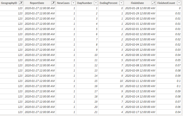Germany Expanded Yes, it’s odd to see a fractional person in the Finished Count. It’s a model and works best in aggregate!

We could stop here, but there is an edge-case that we need to account for. This table will extend beyond the last Report Date loaded. The result will look like everyone is finished with the virus and that is not true, unfortunately. To account for this we will find the maximum Report Date and filter out any rows with a Finish Date beyond.

 1
 2
 3
 4
 5
 6
 7
 8
 9
10
11
12
13
14
15
16
17
18
19
20
21
22
23


Finished = 
VAR FinishedTableBase = 
    GENERATE(
        CROSSJOIN(
            SELECTCOLUMNS(
                  'Daily Total'
                , "ReportDate", 'Daily Total'[ReportDate]
                , "GeographyID", 'Daily Total'[GeographyID]
                , "NewCases", 'Daily Total'[NewCases]
            )
            , 'End Distribution'
        ), 
        VAR FinishDate = [ReportDate] + 'End Distribution'[DayNumber]
        VAR FinishedCount = [NewCases] * 'End Distribution'[EndingPercent] / 100
        RETURN ROW(
              "FinishDate", FinishDate
            , "FinishedCount", FinishedCount
        )
    )
VAR MaxReportDate = CALCULATE(MAX('Daily Total'[ReportDate]), ALL('Daily Total'))
VAR FinishedTableFiltered = FILTER(FinishedTableBase, [FinishDate] <= MaxReportDate)
RETURN
FinishedTableFiltered

Line 20 gets the maximum Report Date, removing any filters that may be applied to the Daily Total table. Line 21 then filters the FinishedTableBase by this maximum date. Line 23 is updated to return the new filtered table.

The next step is to reduce this very large table back down as small as we can get it. We can use the GROUPBY function with CURRENTGROUP to accomplish this task.

 1
 2
 3
 4
 5
 6
 7
 8
 9
10
11
12
13
14
15
16
17
18
19
20
21
22
23
24
25
26
27
28


Finished = 
VAR FinishedTableBase = 
    GENERATE(
        CROSSJOIN(
            SELECTCOLUMNS(
                  'Daily Total'
                , "ReportDate", 'Daily Total'[ReportDate]
                , "GeographyID", 'Daily Total'[GeographyID]
                , "NewCases", 'Daily Total'[NewCases]
            )
            , 'End Distribution'
        ), 
        VAR FinishDate = [ReportDate] + 'End Distribution'[DayNumber]
        VAR FinishedCount = [NewCases] * 'End Distribution'[EndingPercent] / 100
        RETURN ROW(
              "FinishDate", FinishDate
            , "FinishedCount", FinishedCount
        )
    )
VAR MaxReportDate = CALCULATE(MAX('Daily Total'[ReportDate]), ALL('Daily Total'))
VAR FinishedTableFiltered = FILTER(FinishedTableBase, [FinishDate] <= MaxReportDate)
RETURN
GROUPBY(
    FinishedTableFiltered
    , [GeographyID]
    , [FinishDate]
    , "FinishedNew", SUMX(CURRENTGROUP(), [FinishedCount])
    )

The real magic here is the CURRENTGROUP function which allows us to sum a virtual column. Normally, the aggregating functions require a column within an actual table but CURRENTGROUP bypasses this restriction (see documentation here). The result is now back down to nearly the same number as the Daily Total table.

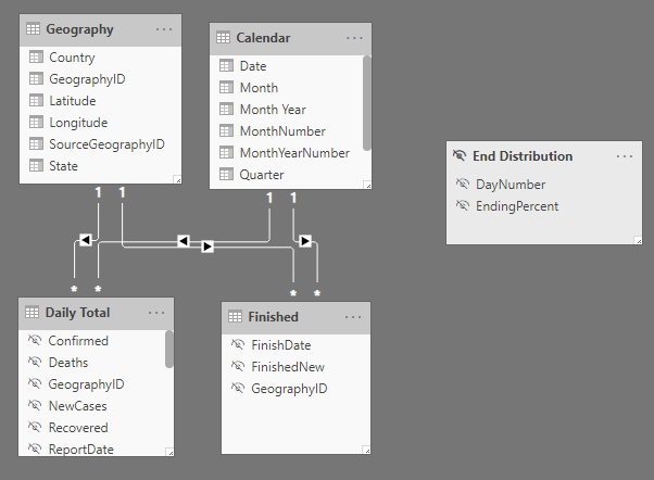
Hide all of the columns in this table and create a relationship between Date[Date] and Finished[FinishDate]. Also create a relationship between Geography[GeographyID] and Finished[GeographyID]. Updated Model

Now let’s write a measure using this new table. Because the FinishedNew count is not a cumulative number, but an additive number and we want to compare it to the total count, it requires special attention.

 1
 2
 3
 4
 5
 6
 7
 8
 9
10
11
12


# Finished (Model) = 
IF(
    MIN('Calendar'[Date]) <= CALCULATE(MAX('Finished'[FinishDate]), ALL('Finished'[FinishDate]))
    ,
        CALCULATE(
            SUM('Finished'[FinishedNew])
            , FILTER(
                ALL('Calendar'[Date])
                , 'Calendar'[Date] <= MAX('Calendar'[Date])
                )
            )
)

This measure sums the FinishedNew column for all dates before the current max date (depending on the row context). This will make sense once we add it to a visual. 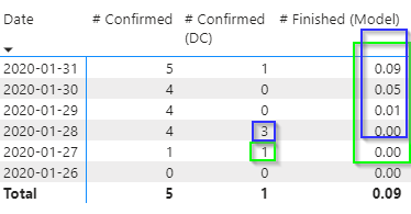Germany Finished Visual The case from 2020-01-27 contributes to the finished count from then for the next 21 days. The three cases on 2020-01-28 contribute to the finished count from then on. In this visual the Report Date is filtered to only what is visible so the Total value is the total of all the numbers prior to the last date in the filter. This effectively gives us a number at the same level of detail as the existing measures.

Now we can subtract it from the # Confirmed to get an active count estimate.

1

# Active (Model) = [# Confirmed] - [# Finished (Model)]

I also prefer to format this field as a whole number because it makes more sense than dealing with fractional people.

How does this new active count compare with existing data? 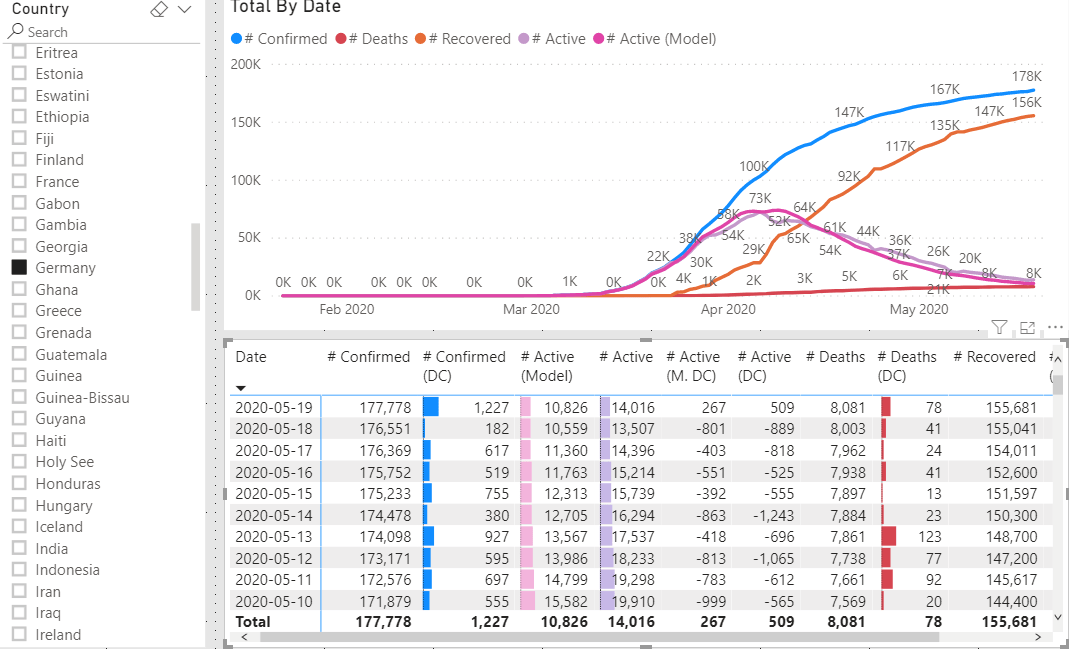New Active Model vs Actual - Germany It seems to be pretty close for Germany.
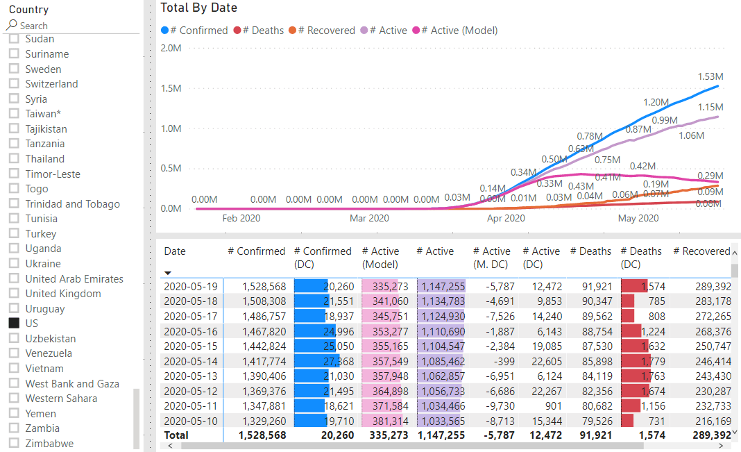New Active Model vs Actual - United States And it helps the situation in the United States look much more positive!

As with all models, it is not perfect. It is only a starting point and seems to give decent values for most situations. As the world begins to open up again it will be interesting to watch this trend and see how the situation is progressing.